CST2013: Optimizer - Interpolation of Primary Data

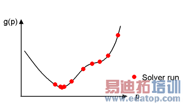
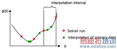
The optimizer supports the interpolation of primary data. The interpolation strategy allows you to significantly reduce the number of actual solver runs. The following two charts demonstrate this behavior by comparing optimizer runs with and without the support of interpolation of primary data. The goalfunction g(p) is plotted versus the parameter value p in both charts.  

Comparison of optimization with and without support of interpolation of primary data

Defining the sample locations

Of course, the result of the optimization depends on the location and the number of the samples. If you use the optimizer with support of interpolation of primary data, you may set the number of samples. Please see the Optimizer Settings page of the optimizer dialog box on  how to select the optimizer with support of primary data.

The location of the samples depend on the number of samples, the initial parameter value that is used upon optimizer start, and the minimum and maximum values a parameter can take. These values can be entered on the Optimizer Settings page of the optimizer dialog box.

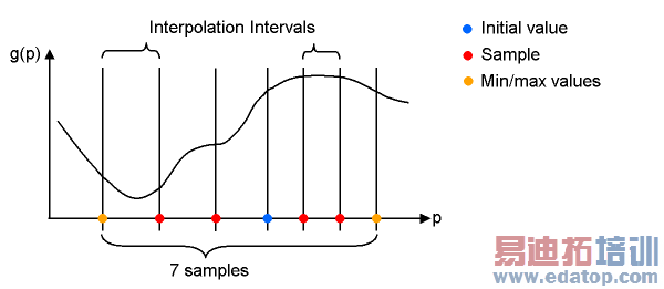
The initial parameter value is always taken as one sample . Therefore, the interpolation intervals to the left and right hand sides of this initial parameter value may be of different size. However, the optimizer tries to locate the samples such that the difference between the interpolation interval sizes on the left and right hand sides of the initial parameter value are as small as possible. Therefore, the initial parameter value may not be located at the middle sample. The following chart shows the different interpolation intervals.

Increasing interpolation accuracy

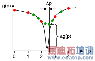
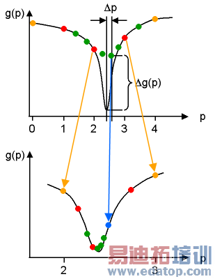
Of course, running the solver at each sample may result in a goal function value that is more accurate than interpolating the primary data and calculating the goal function value out of the interpolated data. If the course of the goal function g(p) shows peaks, the interpolation results may differ from the solver results. The next chart demonstrates this.

This behavior may occur if a small number of samples is taken for a wide parameter range. To increase the interpolation accuracy, you may increase the number of optimizer passes. This causes the optimizer to restart after having found the initial optimum with an internally down-scaled parameter range. The initial parameter value of the additional optimizer run is set to the optimum of the previous optimizer run. The next chart demonstrates this behaviour.